Visual RF Calculators

Open the calculators → · Source on GitHub

It runs in your browser. There’s nothing to install.

Overview

Every input change redraws a picture of the fields, currents or waves next to the number. Every page shows its method and checks itself against published values.

• Skin effect: current density in a round wire from the exact Bessel solution, with animated phase and a flat-conductor view. R_ac/R_dc matches the classic table to within 4e-4, and an independent Kelvin-function (ber/bei) route reproduces the A&S values to 1e-8.
• Coaxial line: radial E and azimuthal H lines, the |E| map, a TEM side view, the TE11 pattern and the 30, 60 and 77 Ω trade-off curves. Checked against cable and connector data (RG-58, RG-402, LMR-400, N, 7/16, 3.5 mm, 2.4 mm), the analytic optima, Wheeler’s rule for loss, and an independent TE11 root solve to 1e-8.
• Microstrip, solved live: a finite-difference Laplace solve of the cross-section in a web worker, with equipotentials, E lines and the mesh. Z0 is within 0.36% of Hammerstad–Jensen over 20 cases (w/h 0.1–10, εr 2.2–12.9), and within 0.16% on the refined grid.
• Rectangular waveguide: TE/TM cross-sections, an animated side view, the mode chart, evanescent decay, vp and vg. Matches Pozar Example 3.1 within 0.3%, and every wall-loss formula agrees with a direct power-loss integration of the fields to within 0.2%.
• Path loss and link budget: spherical spreading and effective aperture, with a waterfall link budget including rain. FSPL follows ITU-R P.525, and rain uses ITU-R P.838-3, whose Table 5 the code reproduces (k within 0.05%, α within 1e-4).

Tech: each calculator is one self-contained HTML file with vanilla JavaScript and canvas. The Node tests load the maths from the built pages, so they check the code the browser runs.

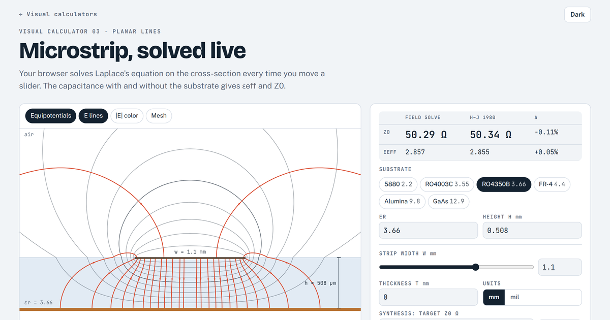The microstrip page: a live field solve next to the Hammerstad–Jensen closed form.