A neural surrogate for MMIC spiral inductors
Problem. This surrogate maps the geometry of a GaAs square spiral to L(f), Q(f) and self-resonant frequency (SRF). The inputs are turns 1.5-5.5, width 5-20 um, spacing 5-15 um and inner diameter 40-200 um. It is benchmarked against held-out HFSS solves.
Data. I built a parametric air-bridge spiral in HFSS 2026 R1 (pyaedt, non-graphical) on a generic textbook GaAs stack: 100 um GaAs and 3 um gold, swept 1-20 GHz, with L and Q taken from Y11. A mesh study set the solve: within 0.3% (L) and 1.3% (Q) of a 2-4x denser mesh. The default mesh read Q 7-11% low. I ran 240 Latin-hypercube designs with no failures: 7.6 h, 112 s per solve.
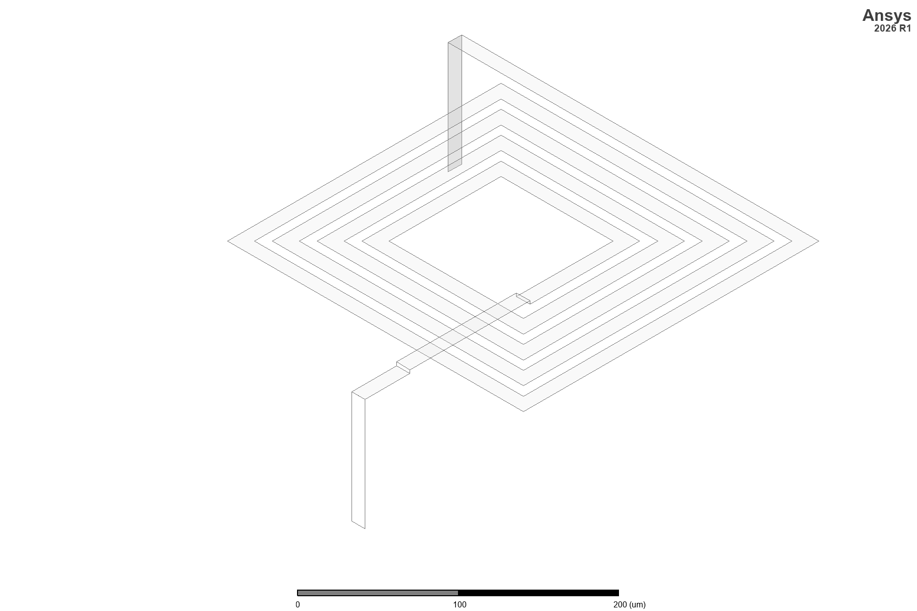 The parametric air-bridge spiral in HFSS. All results on this page are simulated: HFSS against HFSS, on a generic textbook GaAs stack.
Model. A 5-seed MLP ensemble, pointwise in (geometry, f). It takes closed-form physics features as inputs and predicts the log correction to Wheeler. A geometry-only MLP and gradient boosting serve as cross-checks. 20% of designs (49) were held out, stratified.
Results (held-out designs, f < 0.8 SRF):
| L MAPE | Q MAPE | |
|---|---|---|
| Physics-feature MLP | 1.5% (P95 3.9%) | 1.1% (P95 3.1%) |
| Geometry-only MLP | 3.1% | 2.3% |
| Gradient boosting | 3.9% | 3.2% |
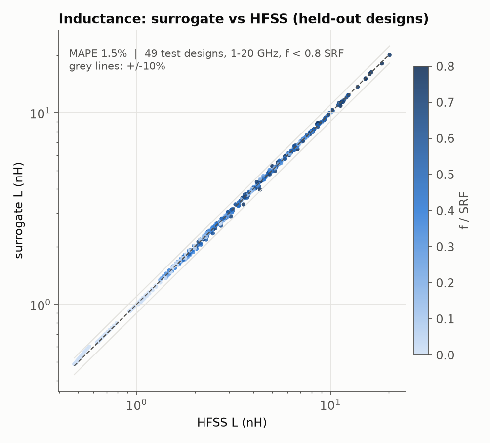 Inductance, surrogate against HFSS on the 49 held-out designs (simulated).
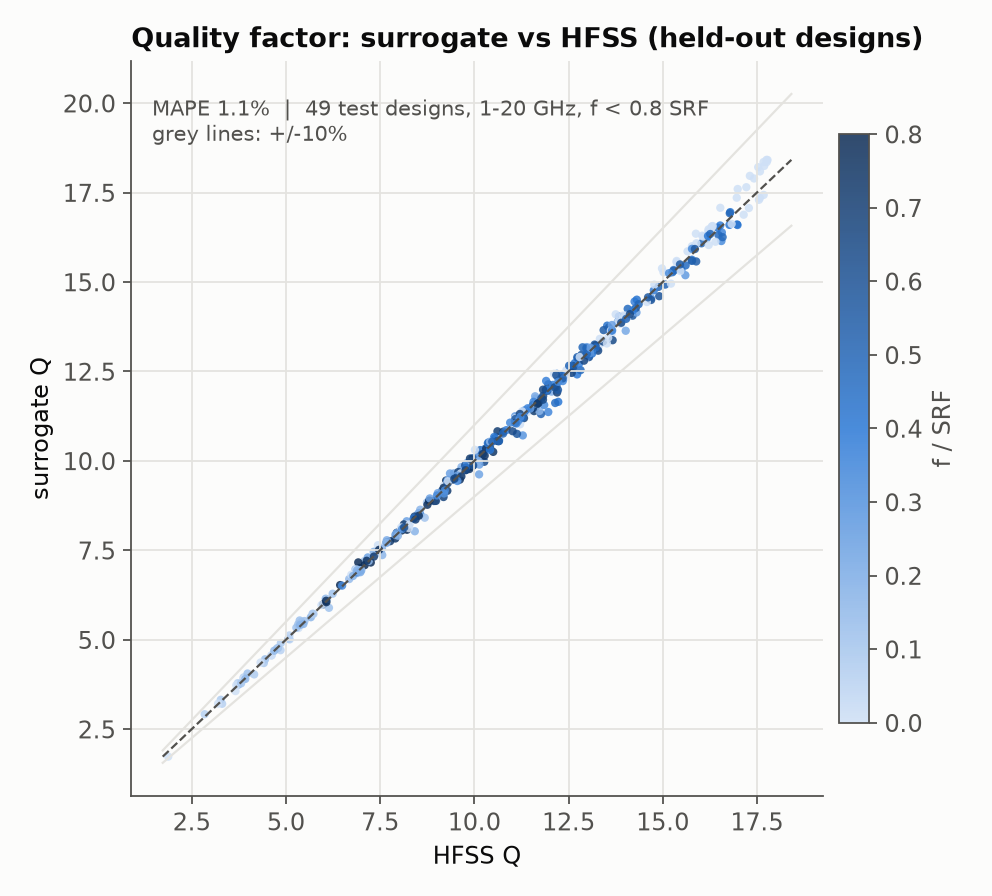 Quality factor, surrogate against HFSS on the same held-out designs (simulated).
- At 1 GHz: 1.0% L error, against 14.5% for modified Wheeler (Mohan 1999) and 8.2% for Wheeler plus a lead correction.
- SRF: 0.7% error, against 20% for a pi-model baseline.
- Speed: 0.6 ms per prediction, about 180,000x faster than a solve.
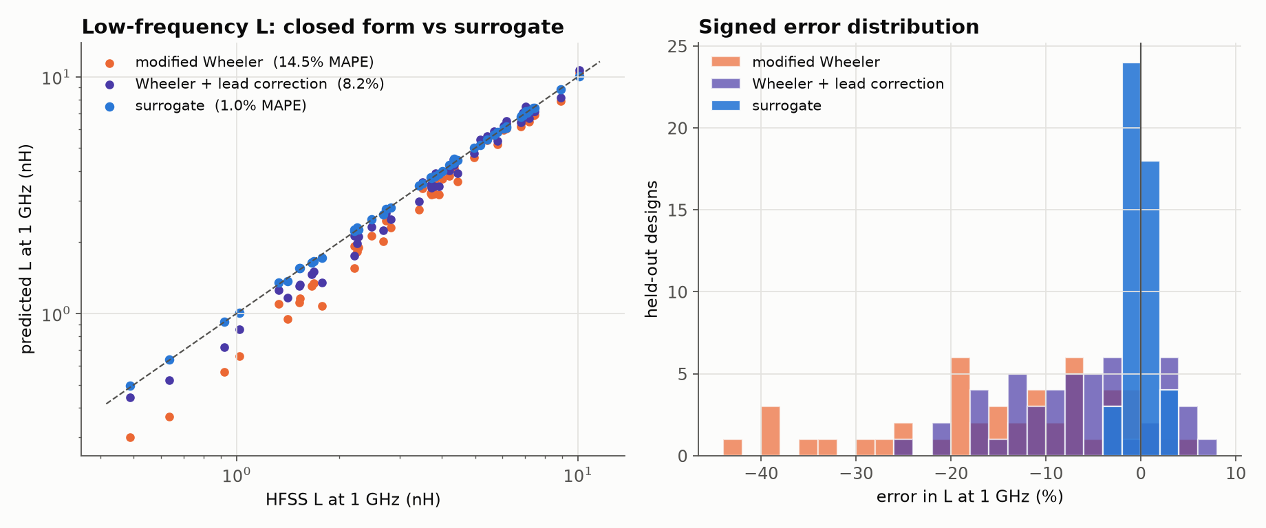 Inductance at 1 GHz: the surrogate against modified Wheeler and Wheeler with a lead correction, on the held-out designs.
Where it degrades.
- Near resonance (0.9-0.95 SRF) the error rises to 4.6% (L) and 4.9% (Q).
- The worst design (8.3%) sits at a corner of the box.
- Trained on N <= 4.5 and tested above it, the physics-feature MLP holds at 1.6% (L) and 1.4% (Q). The geometry-only MLP gets 4.4% and 4.7%.
- Q’s 1.1% is at HFSS’s own mesh-noise floor.
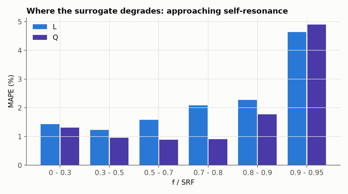 Where the surrogate degrades: error by fraction of the self-resonant frequency.
Inverse design. Spec: 2.0 nH at 10 GHz with Q >= 16. The best training design reached only Q 14.4. The surrogate scored 200,000 geometries in 6 s. One HFSS check of its pick gave Q 16.2 (met) and an SRF within 0.8% of the prediction. L came out 1.92 nH, 4% short of the target. The optimizer chose an edge-of-box design where the model reads optimistic, and the ensemble spread did not flag it. The next step is an HFSS-in-the-loop iteration.
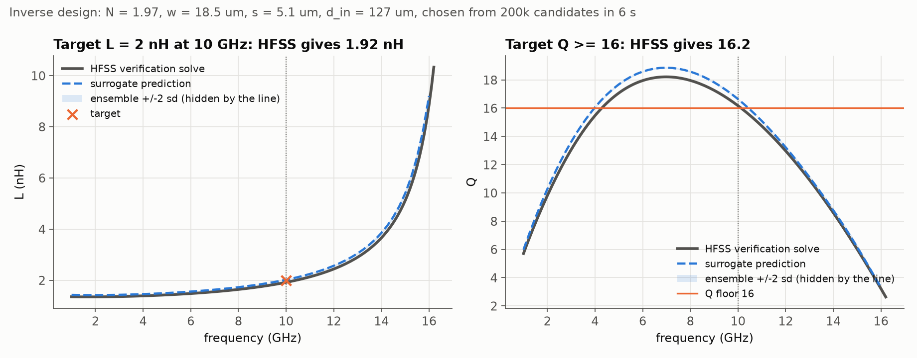 Inverse design: the surrogate’s pick against one HFSS verification solve. Q met the floor; L came out 4 % short.